Tutorial 01: Start with pyTENAX

Import all libraries needed for running basic TENAX

from importlib.resources import files
import numpy as np
import pandas as pd
import matplotlib.pyplot as plt
# Import pyTENAX
from pyTENAX import tenax, plotting

Let’s initiate TENAX class with given setup. For more information about TENAX class, please refer to API documention.

# Initiate TENAX class with customized setup
S = tenax.TENAX(
    return_period=[
        2,
        5,
        10,
        20,
        50,
        100,
        200,
    ],
    durations=[10, 60, 180, 360, 720, 1440], #durations are in minutes and they refer to depth of rainfall within given duration
    time_resolution=10,  # time resolution in minutes
    left_censoring=[0, 0.90], # left censoring threshold
    alpha=0.05, # dependence of shape on T depends on statistical significance at the alpha-level.
    min_rain = 0.1, # minimum rainfall depth threshold
)

Load test data included in the resources directory.

The column names of the precipitation and temperature datasets need to be specified for the TENAX preprocessing stage. The indexes also need to be set to datetime.

# Load precipitation data
# Create input path file for the test file
file_path_input = files('pyTENAX.res').joinpath('prec_data_Aadorf.parquet')
# Load data from csv file
data = pd.read_parquet(file_path_input)
# Convert 'prec_time' column to datetime, if it's not already
data["prec_time"] = pd.to_datetime(data["prec_time"])
# Set 'prec_time' as the index
data.set_index("prec_time", inplace=True)
name_col = "prec_values"  # name of column containing data to extract

# Load temperature data
file_path_temperature = files('pyTENAX.res').joinpath('temp_data_Aadorf.parquet')
t_data = pd.read_parquet(file_path_temperature)
# Convert 'temp_time' column to datetime if it's not already in datetime format
t_data["temp_time"] = pd.to_datetime(t_data["temp_time"])
# Set 'temp_time' as the index
t_data.set_index("temp_time", inplace=True)
temp_name_col = "temp_values"

Preprocessing

Remove incomplete years. Default is 10%.

This can be changed in TENAX class initiation by including “tolerance” parameter.

tolerance (float, optional): Maximum allowed fraction of missing data in one year. If exceeded, year will be disregarded from samples.

data = S.remove_incomplete_years(data, name_col)

Transfer data from pandas to numpy as some parts of TENAX class doesn’t support pandas, also numpy is faster :)

# get data from pandas to numpy array
df_arr = np.array(data[name_col])
df_dates = np.array(data.index)
df_arr_t_data = np.array(t_data[temp_name_col])
df_dates_t_data = np.array(t_data.index)

Separate rainfall events by dry spell duration of 24h.

If shorter or longer separation time is needed, it can be changed by inlcuding “storm_separation_time” in TENAX class initiation.

# extract indexes of ordinary events
# these are time-wise indexes =>returns list of np arrays with np.timeindex
idx_ordinary = S.get_ordinary_events(data=df_arr,
                                     dates=df_dates,
                                     name_col=name_col,
                                     check_gaps=False)

Now we know the times of rainfall events, we remove events that are too short.

This is done by min_event_duration (int, optional): Minimum event duration [min].

Defaults to 30 (minutes).

# get ordinary events by removing too short events
# returns boolean array, dates of OE in TO, FROM format, and count of OE in each years
arr_vals, arr_dates, n_ordinary_per_year = S.remove_short(idx_ordinary)

Finally, we assign the ordinary events values (maximum depth for given durations)

# assign ordinary events values by given durations, values are in depth per duration, NOT in intensity mm/h
dict_ordinary, dict_AMS = S.get_ordinary_events_values(data=df_arr,
                                                       dates=df_dates,
                                                       arr_dates_oe=arr_dates)

After we know ordinary events values and time of maximum depth during the storms,

we can associate temperatures to these events by calculating the temperature averaged during the 24 hours preceeding the rainfall event peak.

The duration averaged over can be changed by including “temp_time_hour” parameter in TENAX class initiation.

dict_ordinary, _, n_ordinary_per_year = S.associate_vars(dict_ordinary,
                                                         df_arr_t_data,
                                                         df_dates_t_data)

The dictionary of ordinary events contains ordinary events and temperature values for all the specified durations.

Here we focus only on 10 minutes depth and extract such from dictionary.

We also calculate the left-censoring threshold.

P = dict_ordinary["10"]["ordinary"].to_numpy()
T = dict_ordinary["10"]["T"].to_numpy()
blocks_id = dict_ordinary["10"]["year"].to_numpy()
# Number of threshold
thr = dict_ordinary["10"]["ordinary"].quantile(S.left_censoring[1])

TENAX model

Here we create temperature intervals for following plots.

eT = np.arange(
    np.min(T)-4, np.max(T) + 4, 1
)  # define T values to calculate distributions. +4 to go beyond graph end

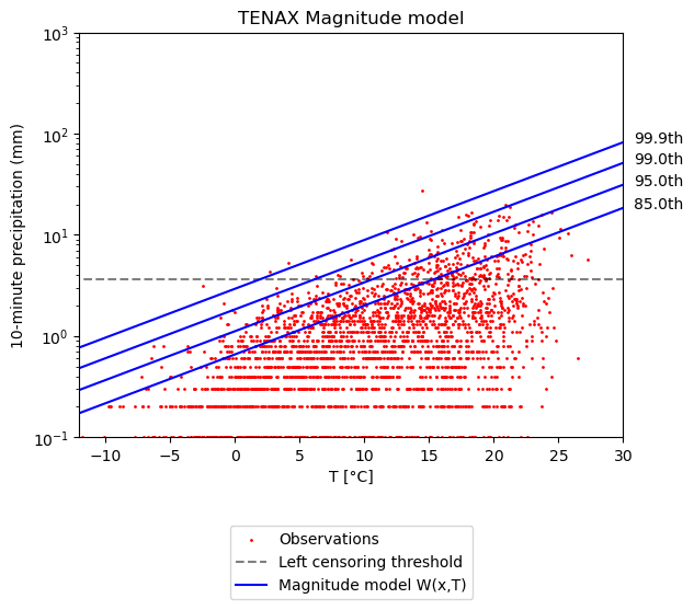
Magnitude model

# magnitude model
F_phat, loglik, _, _ = S.magnitude_model(P, T, thr)

# Plot the magnitude model
qs = [0.85, 0.95, 0.99, 0.999]
plotting.TNX_FIG_magn_model(P, T, F_phat, thr, eT, qs)
plt.ylabel("10-minute precipitation (mm)")
plt.title("TENAX Magnitude model")
plt.legend(loc="upper center", bbox_to_anchor=(0.5, -0.2))
plt.show()

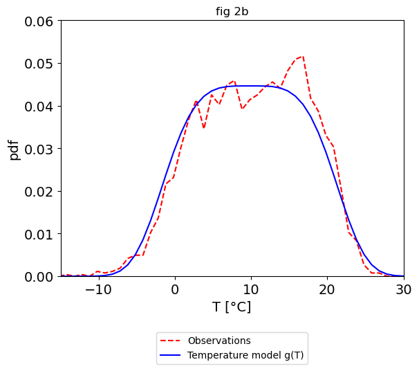
Temperature model

# temperature model
g_phat = S.temperature_model(T)

# Plot the temperature model
hist, pdf_values = plotting.TNX_FIG_temp_model(T, g_phat, S.beta, eT)
plt.title("fig 2b")
plt.legend(loc="upper center", bbox_to_anchor=(0.5, -0.2))
plt.show()

Estimate return levels

We need to create sampling intervals for the Monte Carlo approximation of F(x).

# Sampling intervals for the Montecarlo
Ts = np.arange(np.min(T) - S.temp_delta,
               np.max(T) + S.temp_delta,
               S.temp_res_monte_carlo)

After that we simply call the model_inversion function to estimate return levels based on our Magnitude and Temperature model.

We also estimate TENAX uncertainty using bootstrapping, by creating 100 samples with mixed years. Estimating TENAX uncertainty can take a while as it runs TENAX 100x

#  mean n of ordinary events
n = n_ordinary_per_year.sum() / len(n_ordinary_per_year)

# estimates return levels using MC samples
RL, _, P_check = S.model_inversion(F_phat, g_phat, n, Ts)

# TENAX uncertainty
S.n_monte_carlo = 20000
F_phat_unc, g_phat_unc, RL_unc, n_unc, n_err = S.TNX_tenax_bootstrap_uncertainty(
    P, T, blocks_id, Ts
)

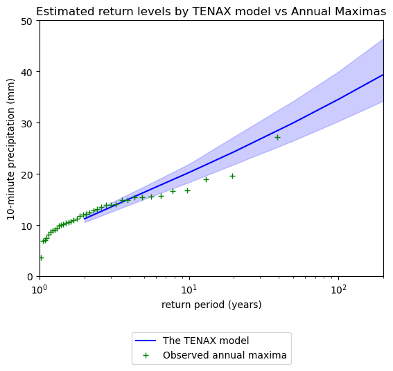
AMS = dict_AMS["10"]  # yet the annual maxima
plotting.TNX_FIG_valid(AMS, S.return_period, RL=RL, RL_unc=RL_unc )
plt.title("Estimated return levels by TENAX model vs Annual Maximas")
plt.ylabel("10-minute precipitation (mm)")
plt.legend(loc="upper center", bbox_to_anchor=(0.5, -0.2))
plt.show()

--- bootstrap_uncertainty internal timings ---
  resample               0.033 s
  magnitude_model        3.019 s
  temperature_model      0.311 s
  model_inversion        2.276 s