Tutorial 03: TENAX Hindcast evaluation

This tutorial guides you through the process of implementing the scaling of TENAX-based changes in mean temperature (𝜇 μ) and the standard deviation of temperature (σ) during precipitation events.

Although this method can also be used to project changes in extreme sub-hourly precipitation under a future warmer climate, it relies solely on climate model projections of temperatures during wet days and anticipated changes in precipitation frequency.”

Import all libraries needed for running TENAX and SMEV

[1]:

from importlib.resources import files
import numpy as np
import pandas as pd
import matplotlib.pyplot as plt
from scipy.stats import chi2
# Import pyTENAX
from pyTENAX import tenax, plotting

Let’s initiate TENAX class and SMEV class with given setup.

[2]:

# Initiate TENAX class with customized setup
S = tenax.TENAX(
    return_period=[
        2,
        5,
        10,
        20,
        50,
        100,
        200,
    ],
    durations=[10, 60, 180, 360, 720, 1440], #durations are in minutes and they refer to depth of rainfall within given duration
    time_resolution=10,  # time resolution in minutes
    left_censoring=[0, 0.90], # left censoring threshold
    alpha=0.05, #dependence of shape on T depends on statistical significance at the alpha-level.
    min_rain = 0.1, #minimum rainfall depth threshold
)

Once again we start with same data.

[3]:

# Load precipitation data
# Create input path file for the test file
file_path_input = files('pyTENAX.res').joinpath('prec_data_Aadorf.parquet')
# Load data from csv file
data = pd.read_parquet(file_path_input)
# Convert 'prec_time' column to datetime, if it's not already
data["prec_time"] = pd.to_datetime(data["prec_time"])
# Set 'prec_time' as the index
data.set_index("prec_time", inplace=True)
name_col = "prec_values"  # name of column containing data to extract

# load temperature data
file_path_temperature = files('pyTENAX.res').joinpath('temp_data_Aadorf.parquet')
t_data = pd.read_parquet(file_path_temperature)
# Convert 'temp_time' column to datetime if it's not already in datetime format
t_data["temp_time"] = pd.to_datetime(t_data["temp_time"])
# Set 'temp_time' as the index
t_data.set_index("temp_time", inplace=True)
temp_name_col = "temp_values"

Repeat the preprocessing to get ordinary events values and corresponding temperature.

We once again focus only on 10-minuts rainfall depth.

[4]:

data = S.remove_incomplete_years(data, name_col)

# get data from pandas to numpy array
df_arr = np.array(data[name_col])
df_dates = np.array(data.index)
df_arr_t_data = np.array(t_data[temp_name_col])
df_dates_t_data = np.array(t_data.index)

# extract indexes of ordinary events
# these are time-wise indexes =>returns list of np arrays with np.timeindex
idx_ordinary = S.get_ordinary_events(data=df_arr,
                                     dates=df_dates,
                                     name_col=name_col,
                                     check_gaps=False)

# get ordinary events by removing too short events
# returns boolean array, dates of OE in TO, FROM format, and count of OE in each years
arr_vals, arr_dates, n_ordinary_per_year = S.remove_short(idx_ordinary)

# assign ordinary events values by given durations, values are in depth per duration, NOT in intensity mm/h
dict_ordinary, dict_AMS = S.get_ordinary_events_values(data=df_arr,
                                                       dates=df_dates,
                                                       arr_dates_oe=arr_dates)

dict_ordinary, _, n_ordinary_per_year = S.associate_vars(dict_ordinary,
                                                         df_arr_t_data,
                                                         df_dates_t_data)

# Your data (P, T arrays) and threshold thr=3.8
P = dict_ordinary["10"]["ordinary"].to_numpy()  # Replace with your actual data
T = dict_ordinary["10"]["T"].to_numpy()  # Replace with your actual data
blocks_id = dict_ordinary["10"]["year"].to_numpy()  # Replace with your actual data
# Number of threshold
thr = dict_ordinary["10"]["ordinary"].quantile(S.left_censoring[1])
# Exctract annual maximas
AMS = dict_AMS["10"]  # yet the annual maxima

# For plotting
# we must create range of temperature
eT = np.arange(
    np.min(T)-4, np.max(T) + 4, 1
)  # define T values to calculate distributions. +4 to go beyond graph end

Hindcast evaluation

We evaluated the ability of the TENAX model to project precipitation return levels under increased temperatures through a hindcast, by splitting the 38-year record of the climate station into two 19-year periods.

[5]:

yrs = dict_ordinary["10"]["oe_time"].dt.year
yrs_unique = np.unique(yrs)
midway = yrs_unique[
    int(np.ceil(np.size(yrs_unique) / 2)) - 1
]  # -1 to adjust indexing because this returns a sort of length

# DEFINE FIRST PERIOD
P1 = P[yrs <= midway]
T1 = T[yrs <= midway]
AMS1 = AMS[AMS["year"] <= midway]
n_ordinary_per_year1 = n_ordinary_per_year[n_ordinary_per_year.index <= midway]
n1 = n_ordinary_per_year1.sum() / len(n_ordinary_per_year1)

# DEFINE SECOND PERIOD
P2 = P[yrs > midway]
T2 = T[yrs > midway]
AMS2 = AMS[AMS["year"] > midway]
n_ordinary_per_year2 = n_ordinary_per_year[n_ordinary_per_year.index > midway]
n2 = n_ordinary_per_year2.sum() / len(n_ordinary_per_year2)

Comparing Temperature models in two periods (1981-1999 & 2000-2018)

[6]:

g_phat1 = S.temperature_model(T1) #returns mu and sigma
g_phat2 = S.temperature_model(T2) #returns mu and sigma

_, _ = plotting.TNX_FIG_temp_model(
    T=T1,
    g_phat=g_phat1,
    beta=4,
    eT=eT,
    obscol="b",
    valcol="b",
    obslabel=None,
    vallabel="Temperature model " + str(yrs_unique[0]) + "-" + str(midway),
)
_, _ = plotting.TNX_FIG_temp_model(
    T=T2,
    g_phat=g_phat2,
    beta=4,
    eT=eT,
    obscol="r",
    valcol="r",
    obslabel=None,
    vallabel="Temperature model " + str(midway + 1) + "-" + str(yrs_unique[-1]),
)  # model based on temp ave and std changes

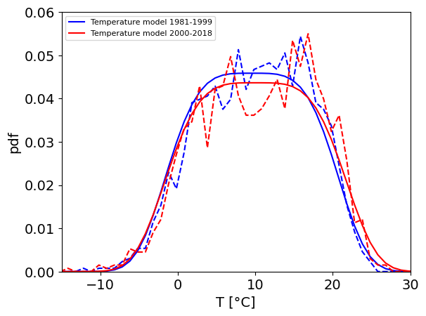
../_images/tutorials_Tutorial_03_12_0.png

Predicted Temperature Model: Based on Changes in μ (Mean) and σ (Standard Deviation)

Increases in the mean temperature (μ) and/or the standard deviation (σ) imply a higher probability of precipitation events occurring at higher temperatures.

mu_delta represents the change in mean temperature during precipitation events.
sigma_factor represents the scaling factor applied to the standard deviation of temperature during precipitation events.

The predicted temperature model is computed by:

Adding mu_delta to the original mean (μ), and
Multiplying the original standard deviation (σ) by sigma_factor.

Mathematical Formulation

Let:

μ = original mean temperature of first model (1981-1999)
σ = original standard deviation of first model (1981-1999)
μ’ = predicted mean temperature
σ’ = predicted standard deviation
Δμ = mu_delta
σ_factor = sigma_factor

Then:

\[\mu' = \mu + \Delta\mu\]

\[\sigma' = \sigma \times \sigma_{\text{factor}}\]

[7]:

mu_delta = np.mean(T2) - np.mean(T1)
sigma_factor = np.std(T2) / np.std(T1)
print(f"Mean temperature has changed by {mu_delta}")
print(f"Standart deviation has changed by factor of {sigma_factor}")

# Create a predicted temperature model
g_phat2_predict = [g_phat1[0] + mu_delta, g_phat1[1] * sigma_factor]

# Compare with Temperatude model of second period we have created before
print(f"Temperatude model of second period {g_phat2}")
print(f"Predicted Temperatude model {g_phat2_predict}")

Mean temperature has changed by 0.48157014197678905
Standart deviation has changed by factor of 1.057753334197546
Temperatude model of second period [10.04413169 12.64035242]
Predicted Temperatude model [10.045000131438464, 12.725393549960536]

Create TENAX Magnitude models of two periods (1981-1999 & 2000-2018)

A magnitude model \(W(x; T)\) was fitted independently for each time period. To assess the similarity of the models, a likelihood ratio test was applied.

According to the general theory of the likelihood ratio test, under the null hypothesis \(H_0\), we compute the likelihood function \(L(\theta)\), where \(\theta \in \Theta\) and \(\Theta\) is the parameter space.

The test statistic is defined as:

\[-2 \ln \left( \frac{\sup_{\theta \in H_0} L(\theta)}{\sup_{\theta \in \Theta} L(\theta)} \right)\]

This statistic follows a chi-squared distribution under certain regularity conditions and can be used to determine whether the models fitted for different periods are significantly different.

[8]:

# Sampling intervals for the Montecarlo based on original temperature T
Ts = np.arange(
    np.min(T) - S.temp_delta, np.max(T) + S.temp_delta, S.temp_res_monte_carlo
)

# Maginitude model of original data that containst both periods (1981-2018)
F_phat, loglik, _, _ = S.magnitude_model(P, T, thr)

# Maginitude model of first period (1981-1999)
F_phat1, loglik1, _, _ = S.magnitude_model(P1, T1, thr)
RL1, _, _ = S.model_inversion(F_phat1, g_phat1, n1, Ts)

# Maginitude model of second period  (2000-2018)
F_phat2, loglik2, _, _ = S.magnitude_model(P2, T2, thr)
RL2, _, _ = S.model_inversion(F_phat2, g_phat2, n2, Ts)

[9]:

if F_phat[1] == 0:  # check if b parameter is 0 (shape=shape_0*b
    dof = 3
    alpha1 = 1  # b parameter is not significantly different from 0; 3 degrees of freedom for the LR test
else:
    dof = 4
    alpha1 = 0  # b parameter is significantly different from 0; 4 degrees of freedom for the LR test

[10]:

# check magnitude model the same in both periods
lambda_LR = -2 * (loglik - (loglik1 + loglik2))
pval = chi2.sf(lambda_LR, dof)
if pval > S.alpha:
    print(f"p={pval}. Magnitude models not  different at {S.alpha*100}% significance.")
else:
    print(f"p={pval}. Magnitude models are different at {S.alpha*100}% significance.")

p=0.6803400017045984. Magnitude models not  different at 5.0% significance.

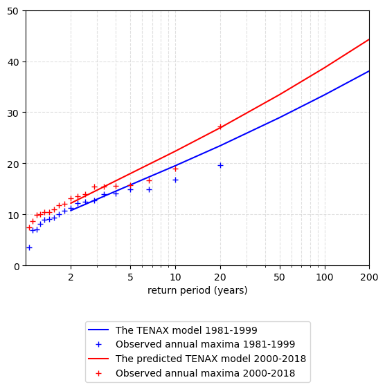
Estimating return levels based on projected change in temperature model and by using the magnitude model of first period.

We compare these return levels to annual maxima of second period and Note: Here we do not apply scaling of n (the average number of events per year). Although, this can be simply done by calculating ratio difference of events during two periods and multipying n1 by this factor.

[11]:

RL2_predict, _, _ = S.model_inversion(F_phat1, g_phat2_predict, n1, Ts)

[12]:

# Plot the results
plotting.TNX_FIG_valid(
    AMS1,
    S.return_period,
    RL1,
    TENAXcol="b",
    obscol_shape="b+",
    TENAXlabel="The TENAX model " + str(yrs_unique[0]) + "-" + str(midway),
    obslabel="Observed annual maxima " + str(yrs_unique[0]) + "-" + str(midway),
)
plotting.TNX_FIG_valid(
    AMS2,
    S.return_period,
    RL2_predict,
    TENAXcol="r",
    obscol_shape="r+",
    TENAXlabel="The predicted TENAX model "
    + str(midway + 1)
    + "-"
    + str(yrs_unique[-1]),
    obslabel="Observed annual maxima " + str(midway + 1) + "-" + str(yrs_unique[-1]),
)
plt.xticks(S.return_period)
plt.gca().set_xticks(S.return_period)  # This sets the actual tick marks on log scale
plt.gca().get_xaxis().set_major_formatter(plt.ScalarFormatter())  # Optional: shows ticks as plain numbers
plt.legend(loc="upper center", bbox_to_anchor=(0.5, -0.2))
plt.grid(True, which='both', axis='both', linestyle='--', color='lightgray', alpha=0.7)
plt.show()

../_images/tutorials_Tutorial_03_21_0.png