Tutorial 04: Simplified Metastatistical Extreme Value formulation (SMEV)

This tutorial introduces the SMEV (Simplified Metastatistical Extreme Value formulation) framework as implemented in pyTENAX.smev.

SMEV is an extreme-value model that fits a Weibull distribution to ordinary precipitation events (not only annual maxima) and extrapolates return levels for multiple durations.

Reference:

Francesco Marra, Davide Zoccatelli, Moshe Armon, Efrat Morin.

A simplified MEV formulation to model extremes emerging from multiple nonstationary underlying processes.

Advances in Water Resources, 127, 280–290, 2019.

https://doi.org/10.1016/j.advwatres.2019.04.002

Key steps covered:

Initialise the SMEV class
Load and preprocess precipitation data
Extract ordinary events (storm separation)
Assign maximum depths per duration
Fit Weibull parameters and compute return levels
Quantify uncertainty via bootstrapping
Visualise results for all durations

Imports

[1]:

from importlib.resources import files
import numpy as np
import pandas as pd
import matplotlib.pyplot as plt
from pyTENAX import smev

1. Initialise the SMEV class

The SMEV class is configured with:

return_period — list of return periods of interest [years]
durations — list of accumulation durations [minutes]
time_resolution — temporal resolution of the input data [minutes]
min_rain — minimum rainfall threshold; only timesteps at or above this value are considered part of a storm
storm_separation_time — dry-spell duration [hours] that separates two independent storms
min_event_duration — minimum storm length [minutes]; shorter events are discarded
left_censoring — probability range used for Weibull fitting; [0.9, 1] means only the top 10% of events are used

[2]:

S_SMEV = smev.SMEV(
    return_period=[2, 5, 10, 20, 50, 100, 200],
    durations=[10, 60, 180, 360, 720, 1440],
    time_resolution=10,
    min_rain=0.1,
    storm_separation_time=24,
    min_event_duration=30,
    left_censoring=[0.9, 1],
)

2. Load and preprocess precipitation data

We use the Aadorf precipitation dataset included in the package resources.

remove_incomplete_years removes years with more than 10% missing data (controlled by the tolerance parameter). This ensures the ordinary-event sample is not biased by data gaps.

[3]:

file_path_input = files('pyTENAX.res').joinpath('prec_data_Aadorf.parquet')
data = pd.read_parquet(file_path_input)
data["prec_time"] = pd.to_datetime(data["prec_time"])
data.set_index("prec_time", inplace=True)
name_col = "prec_values"

data = S_SMEV.remove_incomplete_years(data, name_col)

# Convert to numpy — SMEV functions require numpy input
df_arr   = np.array(data[name_col])
df_dates = np.array(data.index)

print(f"Data loaded: {len(df_arr)} timesteps, {data.index.year.nunique()} complete years")

Data loaded: 1998576 timesteps, 38 complete years

3. Extract ordinary events

Storm separation

get_ordinary_events groups consecutive timesteps at or above min_rain into independent storm events.

Two events are considered independent if they are separated by at least storm_separation_time hours (24 h here).

Removing short events

remove_short discards events shorter than min_event_duration (30 min).

It returns:

arr_vals — boolean array of kept events
arr_dates — (end, start) timestamps of each kept event
n_ordinary_per_year — count of ordinary events per year, used later as the SMEV rate parameter n

[4]:

idx_ordinary = S_SMEV.get_ordinary_events(
    data=df_arr, dates=df_dates, check_gaps=False
)
print(f"Storms detected: {len(idx_ordinary)}")

arr_vals, arr_dates, n_ordinary_per_year = S_SMEV.remove_short(idx_ordinary)
print(f"Storms kept after duration filter: {len(arr_vals)}")

# n = mean number of ordinary events per year (SMEV rate parameter)
n = (n_ordinary_per_year.sum() / len(n_ordinary_per_year)).item()
print(f"Mean ordinary events per year (n): {n:.2f}")

Storms detected: 2848
Storms kept after duration filter: 2634
Mean ordinary events per year (n): 69.32

4. Assign maximum depths per duration

get_ordinary_events_values computes, for each ordinary event and each duration in S_SMEV.durations, the maximum accumulated depth within a sliding window of that length.

The result is two dictionaries keyed by duration string (e.g. "10", "60", …):

dict_ordinary — DataFrame with columns year, oe_time, ordinary (depth in mm)
dict_AMS — DataFrame with annual maximum series (AMS) per year

The default method="vectorized" uses numpy.convolve. For large datasets, method="njit_parallel" (requires numba) is significantly faster — see the docstring for warmup instructions.

[5]:

dict_ordinary, dict_AMS = S_SMEV.get_ordinary_events_values(
    data=df_arr, dates=df_dates, arr_dates_oe=arr_dates
)

# Quick look at the 10-min ordinary events
dict_ordinary["10"].head()

[5]:

	year	oe_time	ordinary
0	1981	1981-01-04 09:10:00	1.1
1	1981	1981-01-10 13:30:00	0.2
2	1981	1981-01-13 01:40:00	0.4
3	1981	1981-01-19 21:10:00	1.4
4	1981	1981-01-26 08:40:00	0.6

5. Fit SMEV and compute return levels

SMEV fits a Weibull distribution to the ordinary event depths.

Left censoring ([0.9, 1]) means only the top 10% of events enter the OLS regression — this focuses the fit on the upper tail, which is what matters for extreme return levels.

Statistical framework

SMEV models the ordinary event depths as Weibull-distributed:

\[F(x) = 1 - \exp\left[-\left(\frac{x}{\lambda}\right)^{\kappa}\right]\]

where \(\lambda > 0\) is the scale parameter and \(\kappa > 0\) is the shape parameter.

The annual maximum distribution is derived by raising the ordinary-event CDF to the power of \(n\) (mean number of events per year), which follows from the assumption that events in a year are independent:

\[\text{SMEV}(x) = \left[F(x)\right]^n = \left(1 - \exp\left[-\left(\frac{x}{\lambda}\right)^{\kappa}\right]\right)^n\]

Setting \(\text{SMEV}(x_T) = 1 - 1/T\) and inverting yields the return level formula implemented in smev_return_values:

\[\boxed{x_T = \lambda \left(-\ln\left(1 - \left(1 - \frac{1}{T}\right)^{1/n}\right)\right)^{1/\kappa}}\]

where \(\lambda\) is the scale, \(\kappa\) is the shape, \(n\) is the mean number of ordinary events per year, and \(T\) is the return period [years].

Running SMEV

You can run SMEV for a single duration directly:

P = dict_ordinary["10"]["ordinary"].to_numpy()
shape, scale = S_SMEV.estimate_smev_parameters(P, S_SMEV.left_censoring)
RL = S_SMEV.smev_return_values(S_SMEV.return_period, shape, scale, n)

Alternatively, _run_smev_all_durations is a convenience wrapper that iterates over all configured durations at once and returns a summary DataFrame.

[6]:

df_results = S_SMEV._run_smev_all_durations(dict_ordinary, n)
print(df_results.to_string())

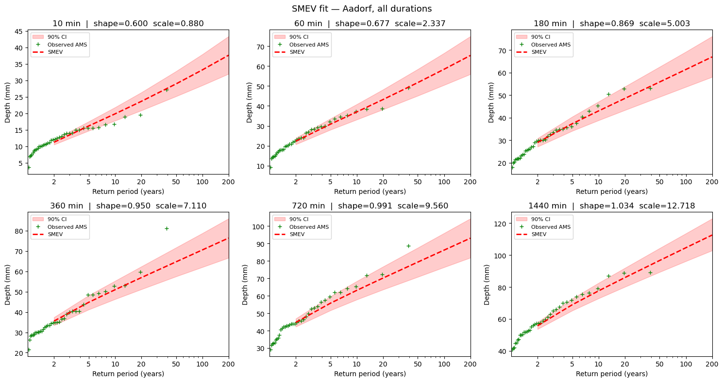
            N_oe  n_mean   shape    scale  RP 2yr  RP 5yr  RP 10yr  RP 20yr  RP 50yr  RP 100yr  RP 200yr
10 min    2634.0   69.32  0.6003   0.8798   11.22   16.17    19.83    23.63    28.93     33.18     37.65
60 min    2634.0   69.32  0.6771   2.3365   22.32   30.86    36.99    43.20    51.70     58.38     65.29
180 min   2634.0   69.32  0.8694   5.0033   29.02   37.34    43.00    48.53    55.81     61.35     66.94
360 min   2634.0   69.32  0.9497   7.1100   35.54   44.77    50.94    56.91    64.67     70.53     76.38
720 min   2634.0   69.32  0.9908   9.5597   44.70   55.77    63.12    70.19    79.35     86.22     93.07
1440 min  2634.0   69.32  1.0340  12.7176   55.76   68.93    77.62    85.92    96.64    104.64    112.60

6. Bootstrap uncertainty

smev_bootstrap_uncertainty estimates the sampling uncertainty of the return levels by block bootstrapping over years.
In each iteration, years are resampled with replacement, the Weibull is refitted, and return levels are recomputed.
The 5th and 95th percentiles of the resulting distribution form the 90% confidence interval (CI).

Note: 1000 iterations × 6 durations takes ~30–60 seconds.

[7]:

boot_results = {}
for dur in [str(d) for d in S_SMEV.durations]:
    P      = dict_ordinary[dur]["ordinary"].to_numpy()
    blocks = dict_ordinary[dur]["year"].to_numpy()
    shape, scale = S_SMEV.estimate_smev_parameters(P, S_SMEV.left_censoring)
    RL     = S_SMEV.smev_return_values(S_SMEV.return_period, shape, scale, n)
    RL_unc = S_SMEV.smev_bootstrap_uncertainty(P, blocks, 1000, n)
    boot_results[dur] = {"shape": shape, "scale": scale, "RL": RL, "RL_unc": RL_unc}

print("Bootstrap complete.")

Bootstrap complete.

7. Visualise: SMEV fit for all durations

Each subplot shows:

Green crosses — observed annual maxima (AMS) at their empirical return periods
Red dashed line — SMEV fitted return level curve
Red shading — 90% bootstrap confidence interval

[8]:

fig, axes = plt.subplots(2, 3, figsize=(15, 8))
axes = axes.flatten()

for ax, dur in zip(axes, [str(d) for d in S_SMEV.durations]):
    AMS    = dict_AMS[dur]
    shape  = boot_results[dur]["shape"]
    scale  = boot_results[dur]["scale"]
    RL     = boot_results[dur]["RL"]
    RL_unc = boot_results[dur]["RL_unc"]

    RL_up  = np.quantile(RL_unc, 0.95, axis=0)
    RL_low = np.quantile(RL_unc, 0.05, axis=0)

    AMS_sort = AMS.sort_values(by=["AMS"])["AMS"]
    plot_pos = np.arange(1, len(AMS_sort) + 1) / (1 + len(AMS_sort))
    eRP = 1 / (1 - plot_pos)

    ax.fill_between(S_SMEV.return_period, RL_low, RL_up, color="r", alpha=0.2, label="90% CI")
    ax.plot(eRP, AMS_sort, "g+", label="Observed AMS")
    ax.plot(S_SMEV.return_period, RL, "--r", linewidth=2, label="SMEV")
    ax.set_xscale("log")
    ax.set_xlim(1, 200)
    ax.set_xticks(S_SMEV.return_period)
    ax.set_xticklabels(S_SMEV.return_period)
    ax.set_xlabel("Return period (years)")
    ax.set_ylabel("Depth (mm)")
    ax.set_title(f"{dur} min  |  shape={shape:.3f}  scale={scale:.3f}")
    ax.legend(fontsize=8)

plt.suptitle("SMEV fit — Aadorf, all durations", fontsize=13)
plt.tight_layout()
plt.show()

../_images/tutorials_Tutorial_04_16_0.png