Tutorial 02: TENAX vs SMEV (extreme value method)

Import all libraries needed for running TENAX and SMEV

from importlib.resources import files
import numpy as np
import pandas as pd
import matplotlib.pyplot as plt
# Import pyTENAX
from pyTENAX import tenax, smev, plotting

Let’s initiate TENAX class and SMEV class with given setup.

# Initiate TENAX class with customized setup
S = tenax.TENAX(
    return_period=[
        2,
        5,
        10,
        20,
        50,
        100,
        200,
    ],
    durations=[10, 60, 180, 360, 720, 1440], #durations are in minutes and they refer to depth of rainfall within given duration
    time_resolution=10,  # time resolution in minutes
    left_censoring=[0, 0.90], # left censoring threshold
    alpha=0.05, #dependence of shape on T depends on statistical significance at the alpha-level.
    min_rain = 0.1, #minimum rainfall depth threshold
)

# Initiate SMEV class with customized setup following TENAX
S_SMEV = smev.SMEV(
    return_period=S.return_period,
    durations=S.durations,
    time_resolution=5,  # time resolution in minutes
    min_rain=0.1,
    storm_separation_time=24,
    min_event_duration=30,
    left_censoring=[S.left_censoring[1], 1],
)

Load same test data as in Tutorial 01.

# Load precipitation data
# Create input path file for the test file
file_path_input = files('pyTENAX.res').joinpath('prec_data_Aadorf.parquet')
# Load data from csv file
data = pd.read_parquet(file_path_input)
# Convert 'prec_time' column to datetime, if it's not already
data["prec_time"] = pd.to_datetime(data["prec_time"])
# Set 'prec_time' as the index
data.set_index("prec_time", inplace=True)
name_col = "prec_values"  # name of column containing data to extract

# load temperature data
file_path_temperature = files('pyTENAX.res').joinpath('temp_data_Aadorf.parquet')
t_data = pd.read_parquet(file_path_temperature)
# Convert 'temp_time' column to datetime if it's not already in datetime format
t_data["temp_time"] = pd.to_datetime(t_data["temp_time"])
# Set 'temp_time' as the index
t_data.set_index("temp_time", inplace=True)
temp_name_col = "temp_values"

Repeat the preprocessing from Tutorial 01.

We once again focus only on 10-minute rainfall depth.

data = S.remove_incomplete_years(data, name_col)

# get data from pandas to numpy array
df_arr = np.array(data[name_col])
df_dates = np.array(data.index)
df_arr_t_data = np.array(t_data[temp_name_col])
df_dates_t_data = np.array(t_data.index)

# extract indexes of ordinary events
# these are time-wise indexes =>returns list of np arrays with np.timeindex
idx_ordinary = S.get_ordinary_events(data=df_arr,
                                     dates=df_dates,
                                     name_col=name_col,
                                     check_gaps=False)

# get ordinary events by removing too short events
# returns boolean array, dates of OE in TO, FROM format, and count of OE in each years
arr_vals, arr_dates, n_ordinary_per_year = S.remove_short(idx_ordinary)

# assign ordinary events values by given durations, values are in depth per duration, NOT in intensity mm/h
dict_ordinary, dict_AMS = S.get_ordinary_events_values(data=df_arr,
                                                       dates=df_dates,
                                                       arr_dates_oe=arr_dates)

dict_ordinary, _, n_ordinary_per_year = S.associate_vars(dict_ordinary,
                                                         df_arr_t_data,
                                                         df_dates_t_data)

# Your data (P, T arrays) and threshold thr=3.8
P = dict_ordinary["10"]["ordinary"].to_numpy()  # Replace with your actual data
T = dict_ordinary["10"]["T"].to_numpy()  # Replace with your actual data
blocks_id = dict_ordinary["10"]["year"].to_numpy()  # Replace with your actual data
# Number of threshold
thr = dict_ordinary["10"]["ordinary"].quantile(S.left_censoring[1])

Repeat TENAX model (same as Tutorial 01)

Note: This doesn’t run bootstrapping for TENAX uncertainty.

eT = np.arange(
    np.min(T)-4, np.max(T) + 4, 1
)  # define T values to calculate distributions. +4 to go beyond graph end

# magnitude model
F_phat, loglik, _, _ = S.magnitude_model(P, T, thr)

# temperature model
g_phat = S.temperature_model(T)

# Sampling intervals for the Montecarlo
Ts = np.arange(np.min(T) - S.temp_delta,
               np.max(T) + S.temp_delta,
               S.temp_res_monte_carlo)

#  mean n of ordinary events
n = n_ordinary_per_year.sum() / len(n_ordinary_per_year)

# estimates return levels using MC samples
RL, _, P_check = S.model_inversion(F_phat, g_phat, n, Ts)

SMEV model

# estimate shape and  scale parameters of weibull distribution
smev_shape, smev_scale = S_SMEV.estimate_smev_parameters(P, S_SMEV.left_censoring)
# estimate return period (quantiles) with SMEV
smev_RL = S_SMEV.smev_return_values(
    S_SMEV.return_period, smev_shape, smev_scale, n.item()
)

smev_RL_unc = S_SMEV.smev_bootstrap_uncertainty(P, blocks_id, S.niter_smev, n.item())

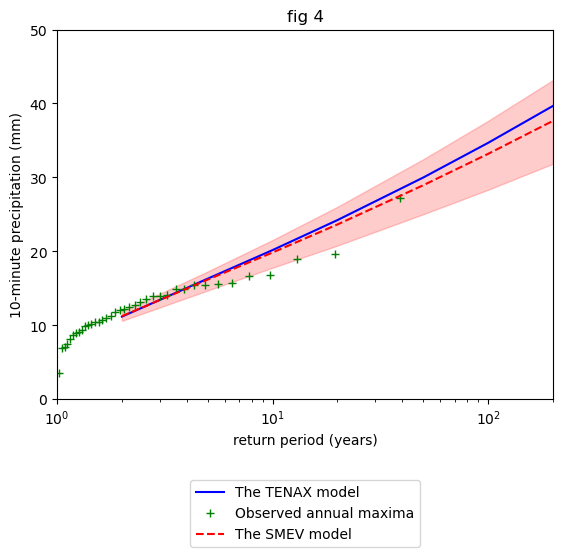
Plot results TENAX vs SMEV

Note, we excluded TENAX uncertainty here as it would take too long to run.

AMS = dict_AMS["10"]  # yet the annual maxima
plotting.TNX_FIG_valid(AMS,
                       S.return_period,
                       RL=RL,
                       smev_RL=smev_RL,
                       RL_unc=[],
                       smev_RL_unc=smev_RL_unc)
plt.title("fig 4")
plt.ylabel("10-minute precipitation (mm)")
plt.legend(loc="upper center", bbox_to_anchor=(0.5, -0.2))
plt.show()

Plot above represents how well TENAX fits extreme value method which does not use temperature as covariate.